This C++ version of BAT is still being maintained, but addition of new features is unlikely. Check out our new incarnation, BAT.jl, the Bayesian analysis toolkit in Julia. In addition to Metropolis-Hastings sampling, BAT.jl supports Hamiltonian Monte Carlo (HMC) with automatic differentiation, automatic prior-based parameter space transformations, and much more. See the BAT.jl documentation.
Results of performance testing for BAT version 0.4.3
Back to | overview for 0.4.3 | all versions |
Test "1d_binomial_2_3"
| Results | |
|---|---|
| Status | good |
| CPU time | 289.7 s |
| Real time | 290.2 s |
| Plots | 1d_binomial_2_3.ps |
| Log | 1d_binomial_2_3.log |
| Settings | |
|---|---|
| N chains | 10 |
| N lag | 10 |
| Convergence | true |
| N iterations (pre-run) | 1000 |
| N iterations (run) | 10000000 |
 |  |  |
| Auto-correlation for the parameter. | Distribution from MCMC and analytic function. | Distribution from MCMC and analytic function in log-scale. |
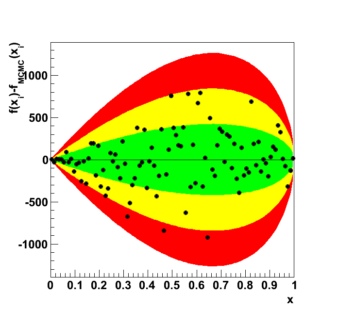 | 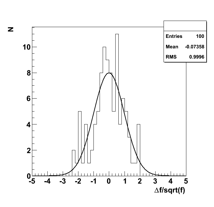 | 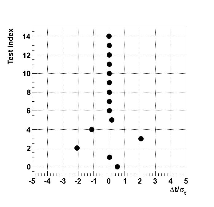 |
| Difference between the distribution from MCMC and the analytic function. The one, two and three sigma uncertainty bands are colored green, yellow and red, respectively. | Pull between the distribution from MCMC and the analytic function. The Gaussian has a mean value of 0 and a standard deviation of 1 (not fitted). | Summary of subtest values. |
| Subtest | Status | Target | Test | Uncertainty | Deviation [%] | Deviation [sigma] | Tol. (Good) | Tol. (Acceptable) | Tol. (Bad) |
|---|---|---|---|---|---|---|---|---|---|
| correlation par 0 | off | 0 | 0.05263 | 0.005176 | - | -10.17 | 0.3 | 0.5 | 0.7 |
| chi2 | good | 100 | 100.5 | 14.14 | 0.4589 | -0.03245 | 42.43 | 70.71 | 98.99 |
| KS | good | 1 | 0.3409 | 0.95 | -65.91 | 0.6938 | 0.95 | 0.99 | 0.9999 |
| mean | good | 0.6 | 0.6001 | 6.223e-05 | 0.02134 | -2.057 | 0.0001867 | 0.0003111 | 0.0004356 |
| mode | good | 0.6667 | 0.655 | 0.0103 | -1.75 | 1.132 | 0.03091 | 0.05151 | 0.07212 |
| variance | good | 0.04 | 0.04078 | 0.004694 | 1.947 | -0.1659 | 0.01408 | 0.02347 | 0.03286 |
| quantile10 | good | 0.3205 | 0.3207 | 0.03333 | 0.0836 | -0.008037 | 0.1 | 0.1667 | 0.2333 |
| quantile20 | good | 0.4175 | 0.4178 | 0.03333 | 0.05738 | -0.007187 | 0.1 | 0.1667 | 0.2333 |
| quantile30 | good | 0.4916 | 0.4918 | 0.03333 | 0.05402 | -0.007966 | 0.1 | 0.1667 | 0.2333 |
| quantile40 | good | 0.5555 | 0.5556 | 0.03333 | 0.02512 | -0.004186 | 0.1 | 0.1667 | 0.2333 |
| quantile50 | good | 0.6143 | 0.6143 | 0.03333 | 0.01117 | -0.002059 | 0.1 | 0.1667 | 0.2333 |
| quantile60 | good | 0.6708 | 0.6709 | 0.03333 | 0.01348 | -0.002714 | 0.1 | 0.1667 | 0.2333 |
| quantile70 | good | 0.7276 | 0.7277 | 0.03333 | 0.005584 | -0.001219 | 0.1 | 0.1667 | 0.2333 |
| quantile80 | good | 0.7877 | 0.7878 | 0.03333 | 0.006262 | -0.00148 | 0.1 | 0.1667 | 0.2333 |
| quantile90 | good | 0.8575 | 0.8575 | 0.03333 | 0.002042 | -0.0005254 | 0.1 | 0.1667 | 0.2333 |
| Subtest | Description |
|---|---|
| correlation par 0 | Calculate the auto-correlation among the points. |
| chi2 | Calculate χ2 and compare with prediction for dof=number of bins with an expectation >= 10. Tolerance good: |χ2-E[χ2]| < 3 · (2 dof)1/2, Tolerance acceptable: |χ2-E[χ2]| < 5 · (2 dof)1/2, Tolerance bad: |χ2-E[χ2]| < 7 · (2 dof)1/2. |
| KS | Calculate the Kolmogorov-Smirnov probability based on the ROOT implemention. Tolerance good: KS prob > 0.05, Tolerance acceptable: KS prob > 0.01 Tolerance bad: KS prob > 0.0001. |
| mean | Compare sample mean, <x>, with expectation value of function, E[x]. Tolerance good: |<x> -E[x]| < 3 · (V[x]/n)1/2,Tolerance acceptable: |<x> -E[x]| < 5 · (V[x]/n)1/2,Tolerance bad: |<x> -E[x]| < 7 · (V[x]/n)1/2. |
| mode | Compare mode of distribution with mode of the analytic function. Tolerance good: |x*-mode| < 3 · V[mode]1/2, Tolerance acceptable: |x*-mode| < 5 · V[mode]1/2 bin widths, Tolerance bad: |x*-mode| < 7 · V[mode]1/2. |
| variance | Compare sample variance s2 of distribution with variance of function. Tolerance good: 3 · V[s2]1/2, Tolerance acceptable: 5 · V[s2]1/2, Tolerance bad: 7 · V[s2]1/2. |
| quantile10 | Compare quantile of distribution from MCMC with the quantile of analytic function. Tolerance good: |q_{X}-E[q_{X}]|<3·V[q]1/2, Tolerance acceptable: |q_{X}-E[q_{X}]|<5·V[q]1/2, Tolerance bad: |q_{X}-E[q_{X}]|<7·V[q]1/2. |
| quantile20 | Compare quantile of distribution from MCMC with the quantile of analytic function. Tolerance good: |q_{X}-E[q_{X}]|<3·V[q]1/2, Tolerance acceptable: |q_{X}-E[q_{X}]|<5·V[q]1/2, Tolerance bad: |q_{X}-E[q_{X}]|<7·V[q]1/2. |
| quantile30 | Compare quantile of distribution from MCMC with the quantile of analytic function. Tolerance good: |q_{X}-E[q_{X}]|<3·V[q]1/2, Tolerance acceptable: |q_{X}-E[q_{X}]|<5·V[q]1/2, Tolerance bad: |q_{X}-E[q_{X}]|<7·V[q]1/2. |
| quantile40 | Compare quantile of distribution from MCMC with the quantile of analytic function. Tolerance good: |q_{X}-E[q_{X}]|<3·V[q]1/2, Tolerance acceptable: |q_{X}-E[q_{X}]|<5·V[q]1/2, Tolerance bad: |q_{X}-E[q_{X}]|<7·V[q]1/2. |
| quantile50 | Compare quantile of distribution from MCMC with the quantile of analytic function. Tolerance good: |q_{X}-E[q_{X}]|<3·V[q]1/2, Tolerance acceptable: |q_{X}-E[q_{X}]|<5·V[q]1/2, Tolerance bad: |q_{X}-E[q_{X}]|<7·V[q]1/2. |
| quantile60 | Compare quantile of distribution from MCMC with the quantile of analytic function. Tolerance good: |q_{X}-E[q_{X}]|<3·V[q]1/2, Tolerance acceptable: |q_{X}-E[q_{X}]|<5·V[q]1/2, Tolerance bad: |q_{X}-E[q_{X}]|<7·V[q]1/2. |
| quantile70 | Compare quantile of distribution from MCMC with the quantile of analytic function. Tolerance good: |q_{X}-E[q_{X}]|<3·V[q]1/2, Tolerance acceptable: |q_{X}-E[q_{X}]|<5·V[q]1/2, Tolerance bad: |q_{X}-E[q_{X}]|<7·V[q]1/2. |
| quantile80 | Compare quantile of distribution from MCMC with the quantile of analytic function. Tolerance good: |q_{X}-E[q_{X}]|<3·V[q]1/2, Tolerance acceptable: |q_{X}-E[q_{X}]|<5·V[q]1/2, Tolerance bad: |q_{X}-E[q_{X}]|<7·V[q]1/2. |
| quantile90 | Compare quantile of distribution from MCMC with the quantile of analytic function. Tolerance good: |q_{X}-E[q_{X}]|<3·V[q]1/2, Tolerance acceptable: |q_{X}-E[q_{X}]|<5·V[q]1/2, Tolerance bad: |q_{X}-E[q_{X}]|<7·V[q]1/2. |