This C++ version of BAT is still being maintained, but addition of new features is unlikely. Check out our new incarnation, BAT.jl, the Bayesian analysis toolkit in Julia. In addition to Metropolis-Hastings sampling, BAT.jl supports Hamiltonian Monte Carlo (HMC) with automatic differentiation, automatic prior-based parameter space transformations, and much more. See the BAT.jl documentation.
Results of performance testing for BAT version 0.9
Back to | overview for 0.9 | all versions |
Test "1d_poisson_5"
| Results | |
|---|---|
| Status | good |
| CPU time | 20.71 s |
| Real time | 20.98 s |
| Plots | 1d_poisson_5.ps |
| Log | 1d_poisson_5.log |
| Settings | |
|---|---|
| N chains | 10 |
| N lag | 10 |
| Convergence | true |
| N iterations (pre-run) | 1000 |
| N iterations (run) | 10000000 |
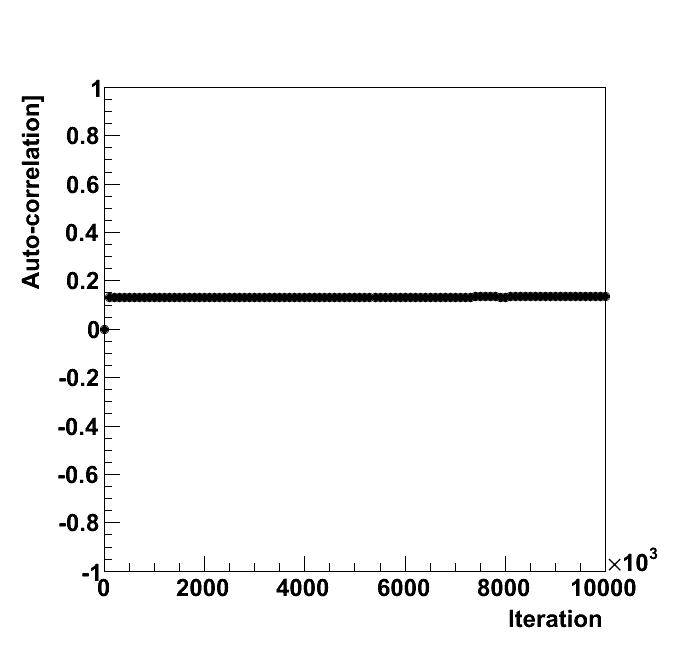 | 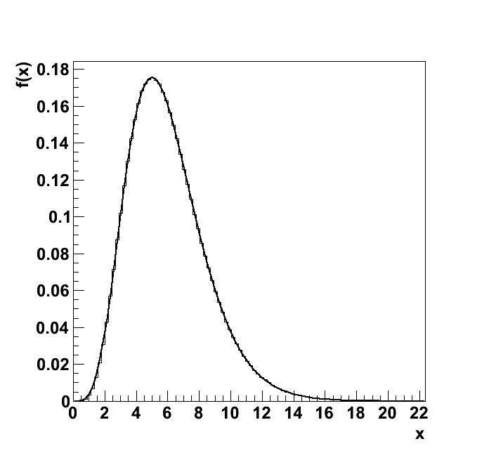 | 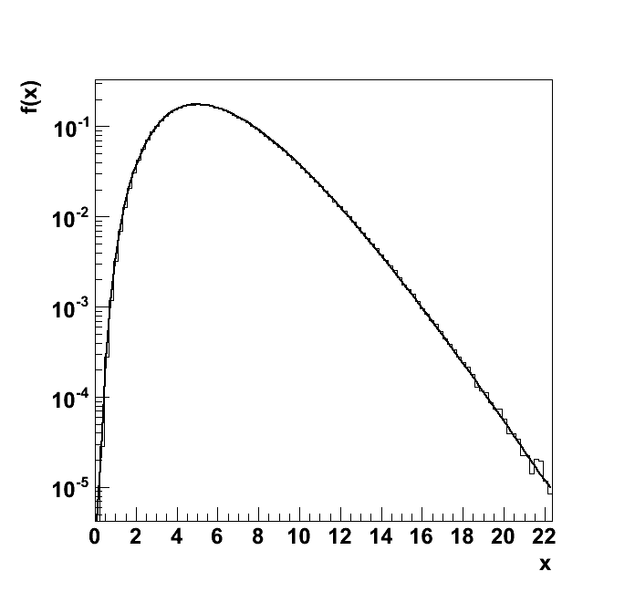 |
| Auto-correlation for the parameter. | Distribution from MCMC and analytic function. | Distribution from MCMC and analytic function in log-scale. |
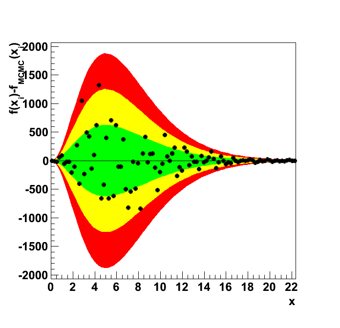 | 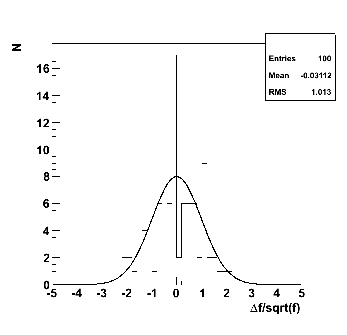 | 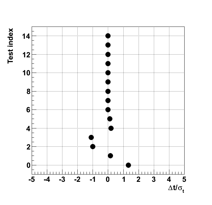 |
| Difference between the distribution from MCMC and the analytic function. The one, two and three sigma uncertainty bands are colored green, yellow and red, respectively. | Pull between the distribution from MCMC and the analytic function. The Gaussian has a mean value of 0 and a standard deviation of 1 (not fitted). | Summary of subtest values. |
| Subtest | Status | Target | Test | Uncertainty | Deviation [%] | Deviation [sigma] | Tol. (Good) | Tol. (Acceptable) | Tol. (Bad) |
|---|---|---|---|---|---|---|---|---|---|
| correlation par 0 | off | 0 | 0.1336 | 0.01319 | - | -10.14 | 0.3 | 0.5 | 0.7 |
| chi2 | good | 99 | 101.2 | 14.07 | 2.203 | -0.155 | 42.21 | 70.36 | 98.5 |
| KS | good | 1 | 0.6793 | 0.95 | -32.07 | 0.3376 | 0.95 | 0.99 | 0.9999 |
| mean | good | 6 | 5.999 | 0.0007736 | -0.0143 | 1.109 | 0.002321 | 0.003868 | 0.005415 |
| mode | good | 5 | 5.031 | 0.1576 | 0.6231 | -0.1976 | 0.4729 | 0.7881 | 1.103 |
| variance | good | 5.996 | 6.119 | 1.037 | 2.044 | -0.1181 | 3.112 | 5.187 | 7.262 |
| quantile10 | good | 3.151 | 3.15 | 0.1576 | -0.01185 | 0.002369 | 0.4729 | 0.7881 | 1.103 |
| quantile20 | good | 3.902 | 3.901 | 0.1576 | -0.02042 | 0.005056 | 0.4729 | 0.7881 | 1.103 |
| quantile30 | good | 4.517 | 4.515 | 0.1576 | -0.03973 | 0.01138 | 0.4729 | 0.7881 | 1.103 |
| quantile40 | good | 5.091 | 5.09 | 0.1576 | -0.02733 | 0.008828 | 0.4729 | 0.7881 | 1.103 |
| quantile50 | good | 5.671 | 5.669 | 0.1576 | -0.02483 | 0.008934 | 0.4729 | 0.7881 | 1.103 |
| quantile60 | good | 6.293 | 6.291 | 0.1576 | -0.0262 | 0.01046 | 0.4729 | 0.7881 | 1.103 |
| quantile70 | good | 7.007 | 7.006 | 0.1576 | -0.02241 | 0.009962 | 0.4729 | 0.7881 | 1.103 |
| quantile80 | good | 7.908 | 7.908 | 0.1576 | -0.004817 | 0.002416 | 0.4729 | 0.7881 | 1.103 |
| quantile90 | good | 9.277 | 9.277 | 0.1576 | -0.003677 | 0.002164 | 0.4729 | 0.7881 | 1.103 |
| Subtest | Description |
|---|---|
| correlation par 0 | Calculate the auto-correlation among the points. |
| chi2 | Calculate χ2 and compare with prediction for dof=number of bins with an expectation >= 10. Tolerance good: |χ2-E[χ2]| < 3 · (2 dof)1/2, Tolerance acceptable: |χ2-E[χ2]| < 5 · (2 dof)1/2, Tolerance bad: |χ2-E[χ2]| < 7 · (2 dof)1/2. |
| KS | Calculate the Kolmogorov-Smirnov probability based on the ROOT implemention. Tolerance good: KS prob > 0.05, Tolerance acceptable: KS prob > 0.01 Tolerance bad: KS prob > 0.0001. |
| mean | Compare sample mean, <x>, with expectation value of function, E[x]. Tolerance good: |<x> -E[x]| < 3 · (V[x]/n)1/2,Tolerance acceptable: |<x> -E[x]| < 5 · (V[x]/n)1/2,Tolerance bad: |<x> -E[x]| < 7 · (V[x]/n)1/2. |
| mode | Compare mode of distribution with mode of the analytic function. Tolerance good: |x*-mode| < 3 · V[mode]1/2, Tolerance acceptable: |x*-mode| < 5 · V[mode]1/2 bin widths, Tolerance bad: |x*-mode| < 7 · V[mode]1/2. |
| variance | Compare sample variance s2 of distribution with variance of function. Tolerance good: 3 · V[s2]1/2, Tolerance acceptable: 5 · V[s2]1/2, Tolerance bad: 7 · V[s2]1/2. |
| quantile10 | Compare quantile of distribution from MCMC with the quantile of analytic function. Tolerance good: |q_{X}-E[q_{X}]|<3·V[q]1/2, Tolerance acceptable: |q_{X}-E[q_{X}]|<5·V[q]1/2, Tolerance bad: |q_{X}-E[q_{X}]|<7·V[q]1/2. |
| quantile20 | Compare quantile of distribution from MCMC with the quantile of analytic function. Tolerance good: |q_{X}-E[q_{X}]|<3·V[q]1/2, Tolerance acceptable: |q_{X}-E[q_{X}]|<5·V[q]1/2, Tolerance bad: |q_{X}-E[q_{X}]|<7·V[q]1/2. |
| quantile30 | Compare quantile of distribution from MCMC with the quantile of analytic function. Tolerance good: |q_{X}-E[q_{X}]|<3·V[q]1/2, Tolerance acceptable: |q_{X}-E[q_{X}]|<5·V[q]1/2, Tolerance bad: |q_{X}-E[q_{X}]|<7·V[q]1/2. |
| quantile40 | Compare quantile of distribution from MCMC with the quantile of analytic function. Tolerance good: |q_{X}-E[q_{X}]|<3·V[q]1/2, Tolerance acceptable: |q_{X}-E[q_{X}]|<5·V[q]1/2, Tolerance bad: |q_{X}-E[q_{X}]|<7·V[q]1/2. |
| quantile50 | Compare quantile of distribution from MCMC with the quantile of analytic function. Tolerance good: |q_{X}-E[q_{X}]|<3·V[q]1/2, Tolerance acceptable: |q_{X}-E[q_{X}]|<5·V[q]1/2, Tolerance bad: |q_{X}-E[q_{X}]|<7·V[q]1/2. |
| quantile60 | Compare quantile of distribution from MCMC with the quantile of analytic function. Tolerance good: |q_{X}-E[q_{X}]|<3·V[q]1/2, Tolerance acceptable: |q_{X}-E[q_{X}]|<5·V[q]1/2, Tolerance bad: |q_{X}-E[q_{X}]|<7·V[q]1/2. |
| quantile70 | Compare quantile of distribution from MCMC with the quantile of analytic function. Tolerance good: |q_{X}-E[q_{X}]|<3·V[q]1/2, Tolerance acceptable: |q_{X}-E[q_{X}]|<5·V[q]1/2, Tolerance bad: |q_{X}-E[q_{X}]|<7·V[q]1/2. |
| quantile80 | Compare quantile of distribution from MCMC with the quantile of analytic function. Tolerance good: |q_{X}-E[q_{X}]|<3·V[q]1/2, Tolerance acceptable: |q_{X}-E[q_{X}]|<5·V[q]1/2, Tolerance bad: |q_{X}-E[q_{X}]|<7·V[q]1/2. |
| quantile90 | Compare quantile of distribution from MCMC with the quantile of analytic function. Tolerance good: |q_{X}-E[q_{X}]|<3·V[q]1/2, Tolerance acceptable: |q_{X}-E[q_{X}]|<5·V[q]1/2, Tolerance bad: |q_{X}-E[q_{X}]|<7·V[q]1/2. |