This C++ version of BAT is still being maintained, but addition of new features is unlikely. Check out our new incarnation, BAT.jl, the Bayesian analysis toolkit in Julia. In addition to Metropolis-Hastings sampling, BAT.jl supports Hamiltonian Monte Carlo (HMC) with automatic differentiation, automatic prior-based parameter space transformations, and much more. See the BAT.jl documentation.
Results of performance testing for BAT version 0.9
Back to | overview for 0.9 | all versions |
Test "1d_poisson_18"
| Results | |
|---|---|
| Status | good |
| CPU time | 21.97 s |
| Real time | 22.2 s |
| Plots | 1d_poisson_18.ps |
| Log | 1d_poisson_18.log |
| Settings | |
|---|---|
| N chains | 10 |
| N lag | 10 |
| Convergence | true |
| N iterations (pre-run) | 1000 |
| N iterations (run) | 10000000 |
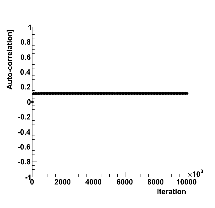 | 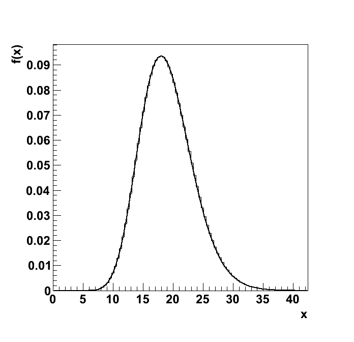 | 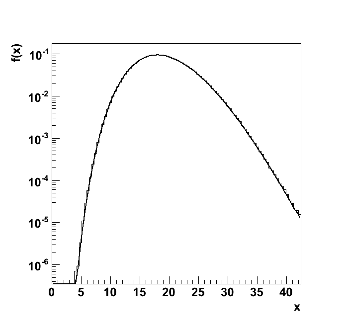 |
| Auto-correlation for the parameter. | Distribution from MCMC and analytic function. | Distribution from MCMC and analytic function in log-scale. |
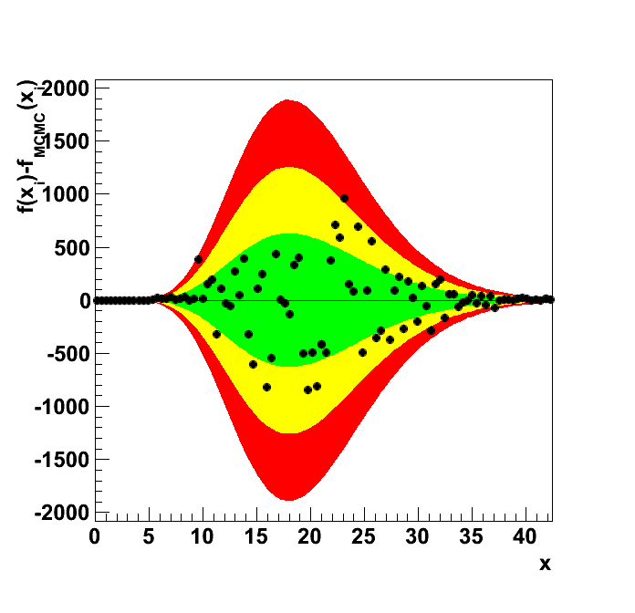 | 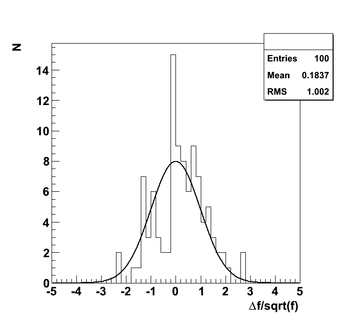 | 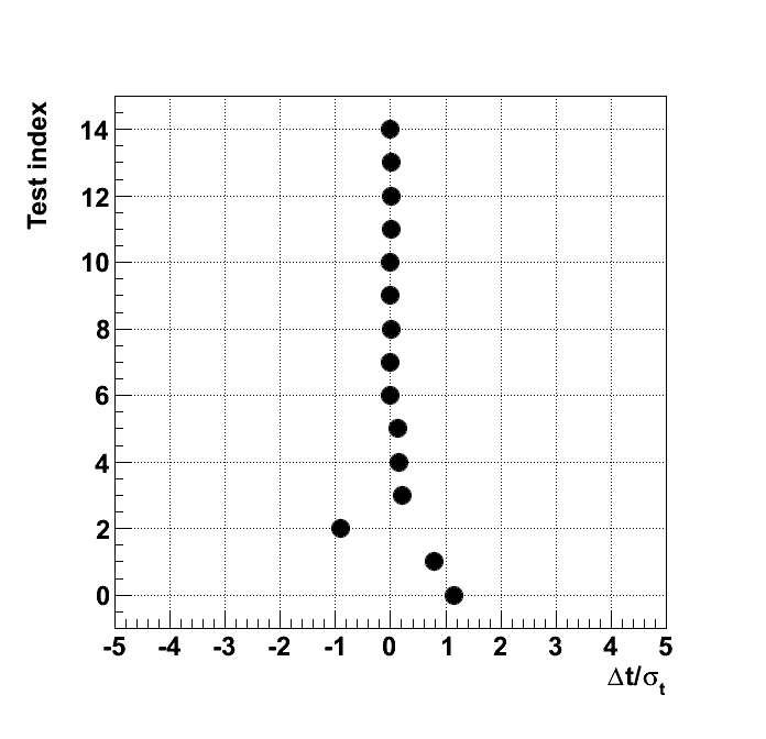 |
| Difference between the distribution from MCMC and the analytic function. The one, two and three sigma uncertainty bands are colored green, yellow and red, respectively. | Pull between the distribution from MCMC and the analytic function. The Gaussian has a mean value of 0 and a standard deviation of 1 (not fitted). | Summary of subtest values. |
| Subtest | Status | Target | Test | Uncertainty | Deviation [%] | Deviation [sigma] | Tol. (Good) | Tol. (Acceptable) | Tol. (Bad) |
|---|---|---|---|---|---|---|---|---|---|
| correlation par 0 | off | 0 | 0.1144 | 0.01136 | - | -10.07 | 0.3 | 0.5 | 0.7 |
| chi2 | good | 89 | 99.51 | 13.34 | 11.8 | -0.7874 | 40.02 | 66.71 | 93.39 |
| KS | good | 1 | 0.7151 | 0.95 | -28.49 | 0.2999 | 0.95 | 0.99 | 0.9999 |
| mean | good | 19 | 19 | 0.001371 | 0.001527 | -0.2116 | 0.004112 | 0.006853 | 0.009594 |
| mode | good | 18 | 18.03 | 0.2171 | 0.1735 | -0.1438 | 0.6514 | 1.086 | 1.52 |
| variance | good | 18.99 | 19.39 | 2.891 | 2.092 | -0.1374 | 8.673 | 14.46 | 20.24 |
| quantile10 | good | 13.67 | 13.66 | 0.2171 | -0.01456 | 0.009166 | 0.6514 | 1.086 | 1.52 |
| quantile20 | good | 15.27 | 15.27 | 0.2171 | -0.004931 | 0.003468 | 0.6514 | 1.086 | 1.52 |
| quantile30 | good | 16.49 | 16.5 | 0.2171 | 0.003618 | -0.002748 | 0.6514 | 1.086 | 1.52 |
| quantile40 | good | 17.6 | 17.6 | 0.2171 | 0.0009216 | -0.0007469 | 0.6514 | 1.086 | 1.52 |
| quantile50 | good | 18.67 | 18.67 | 0.2171 | -0.0002526 | 0.0002172 | 0.6514 | 1.086 | 1.52 |
| quantile60 | good | 19.78 | 19.78 | 0.2171 | 0.003483 | -0.003174 | 0.6514 | 1.086 | 1.52 |
| quantile70 | good | 21.03 | 21.03 | 0.2171 | 0.01556 | -0.01507 | 0.6514 | 1.086 | 1.52 |
| quantile80 | good | 22.54 | 22.54 | 0.2171 | 0.01563 | -0.01623 | 0.6514 | 1.086 | 1.52 |
| quantile90 | good | 24.76 | 24.76 | 0.2171 | -0.003377 | 0.003851 | 0.6514 | 1.086 | 1.52 |
| Subtest | Description |
|---|---|
| correlation par 0 | Calculate the auto-correlation among the points. |
| chi2 | Calculate χ2 and compare with prediction for dof=number of bins with an expectation >= 10. Tolerance good: |χ2-E[χ2]| < 3 · (2 dof)1/2, Tolerance acceptable: |χ2-E[χ2]| < 5 · (2 dof)1/2, Tolerance bad: |χ2-E[χ2]| < 7 · (2 dof)1/2. |
| KS | Calculate the Kolmogorov-Smirnov probability based on the ROOT implemention. Tolerance good: KS prob > 0.05, Tolerance acceptable: KS prob > 0.01 Tolerance bad: KS prob > 0.0001. |
| mean | Compare sample mean, <x>, with expectation value of function, E[x]. Tolerance good: |<x> -E[x]| < 3 · (V[x]/n)1/2,Tolerance acceptable: |<x> -E[x]| < 5 · (V[x]/n)1/2,Tolerance bad: |<x> -E[x]| < 7 · (V[x]/n)1/2. |
| mode | Compare mode of distribution with mode of the analytic function. Tolerance good: |x*-mode| < 3 · V[mode]1/2, Tolerance acceptable: |x*-mode| < 5 · V[mode]1/2 bin widths, Tolerance bad: |x*-mode| < 7 · V[mode]1/2. |
| variance | Compare sample variance s2 of distribution with variance of function. Tolerance good: 3 · V[s2]1/2, Tolerance acceptable: 5 · V[s2]1/2, Tolerance bad: 7 · V[s2]1/2. |
| quantile10 | Compare quantile of distribution from MCMC with the quantile of analytic function. Tolerance good: |q_{X}-E[q_{X}]|<3·V[q]1/2, Tolerance acceptable: |q_{X}-E[q_{X}]|<5·V[q]1/2, Tolerance bad: |q_{X}-E[q_{X}]|<7·V[q]1/2. |
| quantile20 | Compare quantile of distribution from MCMC with the quantile of analytic function. Tolerance good: |q_{X}-E[q_{X}]|<3·V[q]1/2, Tolerance acceptable: |q_{X}-E[q_{X}]|<5·V[q]1/2, Tolerance bad: |q_{X}-E[q_{X}]|<7·V[q]1/2. |
| quantile30 | Compare quantile of distribution from MCMC with the quantile of analytic function. Tolerance good: |q_{X}-E[q_{X}]|<3·V[q]1/2, Tolerance acceptable: |q_{X}-E[q_{X}]|<5·V[q]1/2, Tolerance bad: |q_{X}-E[q_{X}]|<7·V[q]1/2. |
| quantile40 | Compare quantile of distribution from MCMC with the quantile of analytic function. Tolerance good: |q_{X}-E[q_{X}]|<3·V[q]1/2, Tolerance acceptable: |q_{X}-E[q_{X}]|<5·V[q]1/2, Tolerance bad: |q_{X}-E[q_{X}]|<7·V[q]1/2. |
| quantile50 | Compare quantile of distribution from MCMC with the quantile of analytic function. Tolerance good: |q_{X}-E[q_{X}]|<3·V[q]1/2, Tolerance acceptable: |q_{X}-E[q_{X}]|<5·V[q]1/2, Tolerance bad: |q_{X}-E[q_{X}]|<7·V[q]1/2. |
| quantile60 | Compare quantile of distribution from MCMC with the quantile of analytic function. Tolerance good: |q_{X}-E[q_{X}]|<3·V[q]1/2, Tolerance acceptable: |q_{X}-E[q_{X}]|<5·V[q]1/2, Tolerance bad: |q_{X}-E[q_{X}]|<7·V[q]1/2. |
| quantile70 | Compare quantile of distribution from MCMC with the quantile of analytic function. Tolerance good: |q_{X}-E[q_{X}]|<3·V[q]1/2, Tolerance acceptable: |q_{X}-E[q_{X}]|<5·V[q]1/2, Tolerance bad: |q_{X}-E[q_{X}]|<7·V[q]1/2. |
| quantile80 | Compare quantile of distribution from MCMC with the quantile of analytic function. Tolerance good: |q_{X}-E[q_{X}]|<3·V[q]1/2, Tolerance acceptable: |q_{X}-E[q_{X}]|<5·V[q]1/2, Tolerance bad: |q_{X}-E[q_{X}]|<7·V[q]1/2. |
| quantile90 | Compare quantile of distribution from MCMC with the quantile of analytic function. Tolerance good: |q_{X}-E[q_{X}]|<3·V[q]1/2, Tolerance acceptable: |q_{X}-E[q_{X}]|<5·V[q]1/2, Tolerance bad: |q_{X}-E[q_{X}]|<7·V[q]1/2. |