This C++ version of BAT is still being maintained, but addition of new features is unlikely. Check out our new incarnation, BAT.jl, the Bayesian analysis toolkit in Julia. In addition to Metropolis-Hastings sampling, BAT.jl supports Hamiltonian Monte Carlo (HMC) with automatic differentiation, automatic prior-based parameter space transformations, and much more. See the BAT.jl documentation.
Results of performance testing for BAT version 0.9
Back to | overview for 0.9 | all versions |
Test "1d_poisson_10"
| Results | |
|---|---|
| Status | good |
| CPU time | 21.49 s |
| Real time | 21.72 s |
| Plots | 1d_poisson_10.ps |
| Log | 1d_poisson_10.log |
| Settings | |
|---|---|
| N chains | 10 |
| N lag | 10 |
| Convergence | true |
| N iterations (pre-run) | 1000 |
| N iterations (run) | 10000000 |
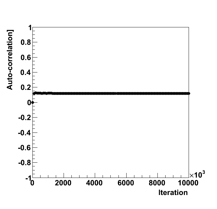 | 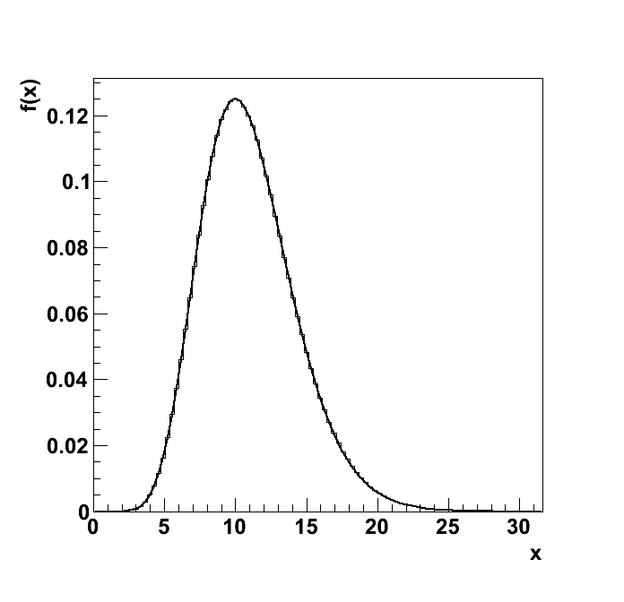 | 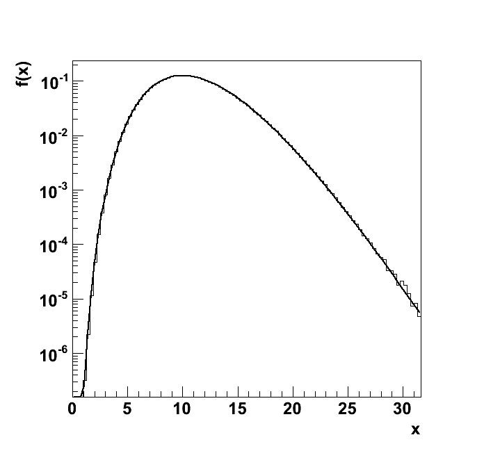 |
| Auto-correlation for the parameter. | Distribution from MCMC and analytic function. | Distribution from MCMC and analytic function in log-scale. |
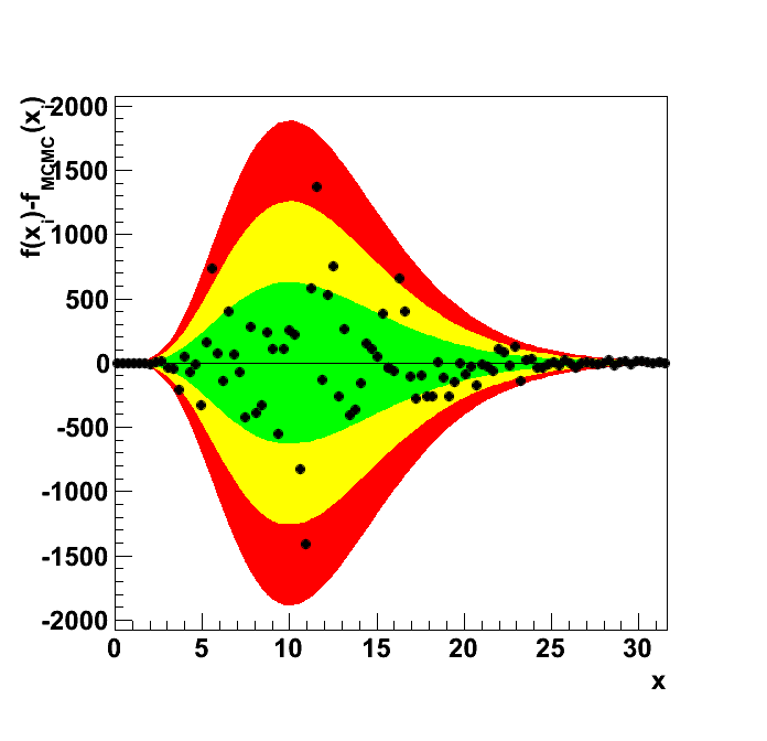 | 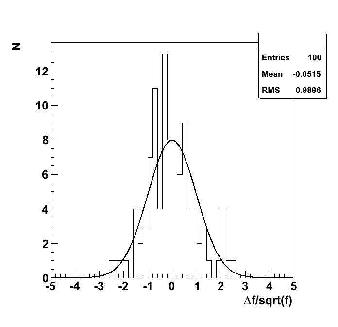 |  |
| Difference between the distribution from MCMC and the analytic function. The one, two and three sigma uncertainty bands are colored green, yellow and red, respectively. | Pull between the distribution from MCMC and the analytic function. The Gaussian has a mean value of 0 and a standard deviation of 1 (not fitted). | Summary of subtest values. |
| Subtest | Status | Target | Test | Uncertainty | Deviation [%] | Deviation [sigma] | Tol. (Good) | Tol. (Acceptable) | Tol. (Bad) |
|---|---|---|---|---|---|---|---|---|---|
| correlation par 0 | off | 0 | 0.1198 | 0.01192 | - | -10.06 | 0.3 | 0.5 | 0.7 |
| chi2 | good | 95 | 98 | 13.78 | 3.154 | -0.2174 | 41.35 | 68.92 | 96.49 |
| KS | good | 1 | 0.9788 | 0.95 | -2.123 | 0.02235 | 0.95 | 0.99 | 0.9999 |
| mean | good | 11 | 11 | 0.001057 | -0.003691 | 0.3842 | 0.00317 | 0.005283 | 0.007397 |
| mode | good | 10 | 9.961 | 0.1874 | -0.3883 | 0.2071 | 0.5623 | 0.9372 | 1.312 |
| variance | good | 11 | 11.21 | 1.757 | 1.974 | -0.1235 | 5.272 | 8.786 | 12.3 |
| quantile10 | good | 7.017 | 7.017 | 0.1874 | -0.01203 | 0.004503 | 0.5623 | 0.9372 | 1.312 |
| quantile20 | good | 8.155 | 8.155 | 0.1874 | -0.001562 | 0.0006794 | 0.5623 | 0.9372 | 1.312 |
| quantile30 | good | 9.049 | 9.049 | 0.1874 | -0.0002559 | 0.0001235 | 0.5623 | 0.9372 | 1.312 |
| quantile40 | good | 9.864 | 9.865 | 0.1874 | 0.002561 | -0.001348 | 0.5623 | 0.9372 | 1.312 |
| quantile50 | good | 10.67 | 10.67 | 0.1874 | 0.003769 | -0.002145 | 0.5623 | 0.9372 | 1.312 |
| quantile60 | good | 11.52 | 11.52 | 0.1874 | 0.007378 | -0.004533 | 0.5623 | 0.9372 | 1.312 |
| quantile70 | good | 12.47 | 12.47 | 0.1874 | -0.004827 | 0.003212 | 0.5623 | 0.9372 | 1.312 |
| quantile80 | good | 13.65 | 13.65 | 0.1874 | -0.005539 | 0.004034 | 0.5623 | 0.9372 | 1.312 |
| quantile90 | good | 15.41 | 15.41 | 0.1874 | -0.01014 | 0.008335 | 0.5623 | 0.9372 | 1.312 |
| Subtest | Description |
|---|---|
| correlation par 0 | Calculate the auto-correlation among the points. |
| chi2 | Calculate χ2 and compare with prediction for dof=number of bins with an expectation >= 10. Tolerance good: |χ2-E[χ2]| < 3 · (2 dof)1/2, Tolerance acceptable: |χ2-E[χ2]| < 5 · (2 dof)1/2, Tolerance bad: |χ2-E[χ2]| < 7 · (2 dof)1/2. |
| KS | Calculate the Kolmogorov-Smirnov probability based on the ROOT implemention. Tolerance good: KS prob > 0.05, Tolerance acceptable: KS prob > 0.01 Tolerance bad: KS prob > 0.0001. |
| mean | Compare sample mean, <x>, with expectation value of function, E[x]. Tolerance good: |<x> -E[x]| < 3 · (V[x]/n)1/2,Tolerance acceptable: |<x> -E[x]| < 5 · (V[x]/n)1/2,Tolerance bad: |<x> -E[x]| < 7 · (V[x]/n)1/2. |
| mode | Compare mode of distribution with mode of the analytic function. Tolerance good: |x*-mode| < 3 · V[mode]1/2, Tolerance acceptable: |x*-mode| < 5 · V[mode]1/2 bin widths, Tolerance bad: |x*-mode| < 7 · V[mode]1/2. |
| variance | Compare sample variance s2 of distribution with variance of function. Tolerance good: 3 · V[s2]1/2, Tolerance acceptable: 5 · V[s2]1/2, Tolerance bad: 7 · V[s2]1/2. |
| quantile10 | Compare quantile of distribution from MCMC with the quantile of analytic function. Tolerance good: |q_{X}-E[q_{X}]|<3·V[q]1/2, Tolerance acceptable: |q_{X}-E[q_{X}]|<5·V[q]1/2, Tolerance bad: |q_{X}-E[q_{X}]|<7·V[q]1/2. |
| quantile20 | Compare quantile of distribution from MCMC with the quantile of analytic function. Tolerance good: |q_{X}-E[q_{X}]|<3·V[q]1/2, Tolerance acceptable: |q_{X}-E[q_{X}]|<5·V[q]1/2, Tolerance bad: |q_{X}-E[q_{X}]|<7·V[q]1/2. |
| quantile30 | Compare quantile of distribution from MCMC with the quantile of analytic function. Tolerance good: |q_{X}-E[q_{X}]|<3·V[q]1/2, Tolerance acceptable: |q_{X}-E[q_{X}]|<5·V[q]1/2, Tolerance bad: |q_{X}-E[q_{X}]|<7·V[q]1/2. |
| quantile40 | Compare quantile of distribution from MCMC with the quantile of analytic function. Tolerance good: |q_{X}-E[q_{X}]|<3·V[q]1/2, Tolerance acceptable: |q_{X}-E[q_{X}]|<5·V[q]1/2, Tolerance bad: |q_{X}-E[q_{X}]|<7·V[q]1/2. |
| quantile50 | Compare quantile of distribution from MCMC with the quantile of analytic function. Tolerance good: |q_{X}-E[q_{X}]|<3·V[q]1/2, Tolerance acceptable: |q_{X}-E[q_{X}]|<5·V[q]1/2, Tolerance bad: |q_{X}-E[q_{X}]|<7·V[q]1/2. |
| quantile60 | Compare quantile of distribution from MCMC with the quantile of analytic function. Tolerance good: |q_{X}-E[q_{X}]|<3·V[q]1/2, Tolerance acceptable: |q_{X}-E[q_{X}]|<5·V[q]1/2, Tolerance bad: |q_{X}-E[q_{X}]|<7·V[q]1/2. |
| quantile70 | Compare quantile of distribution from MCMC with the quantile of analytic function. Tolerance good: |q_{X}-E[q_{X}]|<3·V[q]1/2, Tolerance acceptable: |q_{X}-E[q_{X}]|<5·V[q]1/2, Tolerance bad: |q_{X}-E[q_{X}]|<7·V[q]1/2. |
| quantile80 | Compare quantile of distribution from MCMC with the quantile of analytic function. Tolerance good: |q_{X}-E[q_{X}]|<3·V[q]1/2, Tolerance acceptable: |q_{X}-E[q_{X}]|<5·V[q]1/2, Tolerance bad: |q_{X}-E[q_{X}]|<7·V[q]1/2. |
| quantile90 | Compare quantile of distribution from MCMC with the quantile of analytic function. Tolerance good: |q_{X}-E[q_{X}]|<3·V[q]1/2, Tolerance acceptable: |q_{X}-E[q_{X}]|<5·V[q]1/2, Tolerance bad: |q_{X}-E[q_{X}]|<7·V[q]1/2. |